iEEG
Overview
In this notebook, we will compare data between iEEG contacts inside the hippocapus vs the rest of the brain in terms of band power. We will then extrapolate these band powers across the hippocampus to see if there are systematic differences.
Note that we have already determined which/where channels are in the hippocampus, and preprocessed the iEEG timeseries and converted them to band power values in the ../extras directory. This also included computing power spectrum densities (PSDs) from preprocessed timeseries data, and computing band powers in the below ranges from PSDs. See there for methodological details
[1]:
import numpy as np
import matplotlib.pyplot as plt
import matplotlib.pylab as pl
import nibabel as nib
import hippomaps as hm
import pygeodesic.geodesic as geodesic
from scipy.ndimage import gaussian_filter1d
from brainspace.gradient import GradientMaps
import time
start_time = time.time()
[2]:
# config

# define which subjects and surfaces to examine
den='2mm'
hemis = ['L','R']
labels = ['hipp']#,'dentate']

# get expected number of vertices and their indices
nV,iV = hm.config.get_nVertices(labels,den)

# iEEG parameters
freq = 200 #Hz
bands = ['delta', 'theta', 'alpha', 'beta', 'gamma']
band_lims = np.array([[0.5,4], [4,8], [8,13], [13,30], [30,80]]) # Hz
sampspace = np.arange(0.5,80,0.5)
dist_threshold = 5 # mm
0) Map data to hippocampal surfaces
This tutorial must use checkpoints, because the input data is inconconsistently formatted. See extras/iEEG_Frauscher.ipynb and extras/iEEG_MICs.ipynb for raw and preprocessed data loading.
[3]:
hm.fetcher.get_tutorialCheckpoints(['iEEG_Frauscher_dat.npy', 'iEEG_MICs_dat.npy'])
1) Load the data and examine attributes
Previously we then calculated PSD from each iEEG channel. We then calculated band powers (BP) within 5 bands defined above. Finally, we mapped iEEG channels to hippocampal vertices within 5mm. Thus our hippocampal data is in the shape (number of vertices nV) x (hemispheres 2) x (PSD or number of bands) x (number of channels), where the number of channels is for all channels but data are mostly NaN since most channels are not within 5mm of a hippocampal vertex.
[4]:
# load preprocessed bandpower and periogram data
# all data is all clean channels, hipp dat has non-hippocmapal channels NaN'd out

vars_to_load = ['pxx', 'bp', 'hipp_bp', 'hipp_pxx']
t1 = np.load(f'checkpoints/iEEG_Frauscher_dat.npy',allow_pickle=True)
t2 = np.load(f'checkpoints/iEEG_MICs_dat.npy',allow_pickle=True)
[5]:
PSD = np.concatenate((t1[0], t2[0]),axis=1)
BP = np.concatenate((t1[1], t2[1]),axis=0)
BPhipp = np.concatenate((t1[2],t2[2]),axis=3)
PSDhipp = np.concatenate((t1[3],t2[3]),axis=3)
[6]:
# vertices by hemispheres by bands (band powers) by number of channels
BPhipp.shape
[6]:
(419, 2, 5, 4279)
[7]:
# vertices by hemispheres by bands (band powers) by power spectrum density frequencies
PSDhipp.shape
[7]:
(419, 2, 159, 4279)
Spatial distribution of hippocampal-adjacent channels
[8]:
# find which channels are actually close to any hippocampal vertex

nL = len(np.where(np.any(~np.isnan(BPhipp[:,0,0,:]),axis=0))[0])
nR = len(np.where(np.any(~np.isnan(BPhipp[:,1,0,:]),axis=0))[0])

print('number of L hemis: ' + str(nL))
print('number of R hemis: ' + str(nR))
number of L hemis: 26
number of R hemis: 55
[9]:
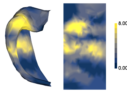
# sum how many channels are close to each vertex
hipp_dat_count = np.sum(~np.isnan(BPhipp),axis=(1,3))[:,0]
hm.plotting.surfplot_canonical_foldunfold(hipp_dat_count, den='2mm', hemis=['L'], labels=labels, unfoldAPrescale=True, tighten_cwindow=True, cmap='cividis', share='row', color_bar='right', embed_nb=True)
/host/percy/local_raid/donna/BrainSpace/brainspace/plotting/base.py:287: UserWarning: Interactive mode requires 'panel'. Setting 'interactive=False'
  warnings.warn("Interactive mode requires 'panel'. "
[9]:
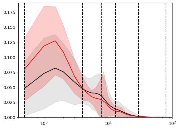
Compare PSDs from the hippocampus to all channels to ensure they are comparable
[10]:
y = np.exp(np.nanmean(np.log(PSD),axis=1))
err = np.nanstd(PSD,axis=1)
plt.plot(sampspace,y,'k')
plt.ylim(0,.19)
plt.fill_between(sampspace, y-err, y+err, alpha=0.2, color='gray')
plt.vlines(band_lims.flatten(),plt.gca().get_ylim()[0],plt.gca().get_ylim()[1],colors='k',linestyles='--')
plt.xscale('log')
plt.xlim(0.4,100)

y = np.exp(np.nanmean(np.log(PSDhipp),axis=(0,1,3)))
err = np.nanstd(PSDhipp,axis=(0,1,3))
plt.plot(sampspace,y,'r')
plt.ylim(0,.19)
plt.fill_between(sampspace, y-err, y+err, alpha=0.2, color='r')
plt.vlines(band_lims.flatten(),plt.gca().get_ylim()[0],plt.gca().get_ylim()[1],colors='k',linestyles='--')
plt.xscale('log')
plt.xlim(0.4,100)
[10]:
(0.4, 100)
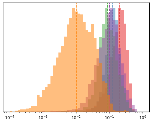
Compare BPs from the hippocampus to all channels to ensure they are comparable
Plot a distribution of band powers from all channels, and from the subset of hippocampal channels
Periodic data is typically log normal distributed, so we apply logarithmic scaling
[11]:
# all channels

colormap = pl.cm.Set1(range(10))
l=['delta', 'theta', 'alpha', 'beta', 'gamma']
fig, ax = plt.subplots()
ax.set_xscale('log')
ax.yaxis.set_visible(False)
ax = [ax]
n=0
cbins = [] # number of channels in each bin
for b in range(5):
    ax = ax + [ax[0].twinx()] # nake a new axis for each distribution so they don't share a y-axis and thus fill the whole plot
    dat = BP[:,b]
    plt.axvline(x=np.nanmedian(dat), color=colormap[n], linestyle='dashed')
    cbins.append(ax[n+1].hist(dat,bins=np.logspace(np.log10(1e-4),np.log10(1), 50), linestyle=None, alpha=0.5,
               color=colormap[b], label=l[b]))
    ax[n+1].yaxis.set_visible(False)
    n=n+1
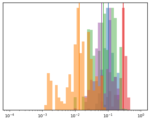
[12]:
# hippocampal channels

colormap = pl.cm.Set1(range(10))
l=['delta', 'theta', 'alpha', 'beta', 'gamma']
fig, ax = plt.subplots()
ax.set_xscale('log')
ax.yaxis.set_visible(False)
ax = [ax]
n=0
hippcbins = [] # number of channels in each bin
for b in range(5):
    ax = ax + [ax[0].twinx()] # nake a new axis for each distribution so they don't share a y-axis and thus fill the whole plot
    dat = BPhipp[:,:,b,:].flatten()
    plt.axvline(x=np.nanmedian(dat), color=colormap[n], linestyle='solid')
    hippcbins.append(ax[n+1].hist(dat,bins=np.logspace(np.log10(1e-4),np.log10(1), 50), linestyle=None, alpha=0.5,
               color=colormap[b], label=l[b]))
    ax[n+1].yaxis.set_visible(False)
    n=n+1
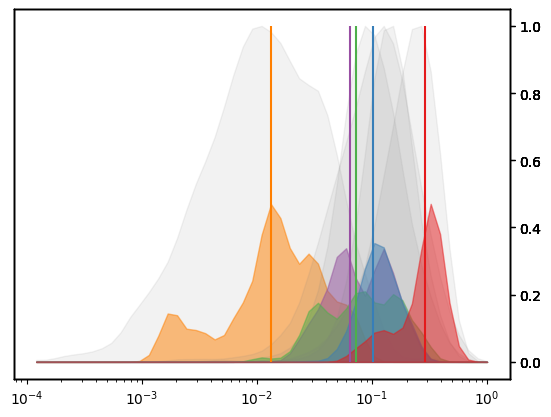
Nicer ridge plot, showing hippocampal data in colour and all data in grey behind
[13]:
colormap = pl.cm.Set1(range(10))
fig, ax = plt.subplots()
ax.set_xscale('log')
ax.yaxis.set_visible(False)
ax = [ax]
sigma = 1
n=0
for b in reversed(range(5)):
    ax = ax + [ax[0].twinx()]
    dat = BP[:,b]
    #ax[n+1].vlines(np.nanmedian(dat),0,1, color='gray', linestyle='dashed')
    plt.fill_between(cbins[b][1][1:],gaussian_filter1d(cbins[b][0],sigma), color='gray', alpha=0.1)
    ax[n+1].yaxis.set_visible(False)
    n=n+1
n=0
for b in reversed(range(5)):
    ax = ax + [ax[0].twinx()]
    dat = BPhipp[:,:,b,:].flatten()
    plt.vlines(np.nanmedian(dat),0,1, color=colormap[b], linestyle='solid')
    ax[n+1].fill_between(hippcbins[b][1][1:],gaussian_filter1d(hippcbins[b][0],sigma), color=colormap[b], alpha=0.5)
    #ax[n+1].hist(dat,bins=np.logspace(np.log10(1e-4),np.log10(1), 50), linestyle=None, alpha=0.5,
    #           color=colormap[b], label=l[b]);
    ax[n+1].yaxis.set_visible(False)
    n=n+1
2) Spatial extrapolation
We can see that simply averaging over all channels doesn’t give a good idea of the spatial distribution of band power, since so much data is missing. Thus, we will extrapolate each channel over the whole hippocampus and then use the distance from the channel as a weighting when performing weighted averaging across channels. See ../extras for an example visualization.
[14]:
gii = nib.load(f'../hippomaps/resources/canonical_surfs/tpl-avg_space-canonical_den-{den}_label-hipp_midthickness.surf.gii')
v = gii.get_arrays_from_intent('NIFTI_INTENT_POINTSET')[0].data
f = gii.get_arrays_from_intent('NIFTI_INTENT_TRIANGLE')[0].data
gii = nib.load(f'../hippomaps/resources/canonical_surfs/tpl-avg_space-canonical_den-{den}_label-dentate_midthickness.surf.gii')
vdg = gii.get_arrays_from_intent('NIFTI_INTENT_POINTSET')[0].data
fdg = gii.get_arrays_from_intent('NIFTI_INTENT_TRIANGLE')[0].data
F = [f, fdg]
V = [v, vdg]
[15]:
weights = np.zeros((BPhipp.shape[0],2,BPhipp.shape[3]))
BPhipp_extrapolated = np.zeros([BPhipp.shape[0],5])
PSDhipp_extrapolated = np.zeros([BPhipp.shape[0],len(PSD)])

for h,hemi in enumerate(hemis):
    for l,label in enumerate(labels):
        for c in range(BPhipp.shape[3]):
            dat = BPhipp[:,h,0,c]
            mask = ~np.isnan(dat[iV[l]])
            if np.any(mask):
                geoalg = geodesic.PyGeodesicAlgorithmExact(V[l], F[l])
                sd,_ = geoalg.geodesicDistances(np.where(mask)[0], None)
                sd = sd**2
                weights[iV[l],h,c] = 1 - (sd/np.max(sd))

totweights = np.nansum(weights, axis=(1,2))
for v in range(weights.shape[0]):
    for h in range(2):
        for c in range(BPhipp.shape[3]):
            w = weights[v,h,c] / totweights[v]
            if w>0:
                BPhipp_extrapolated[v,:] += np.nanmean(BPhipp[:,h,:,c],axis=0) * w
                PSDhipp_extrapolated[v,:] += np.nanmean(PSDhipp[:,h,:,c],axis=0) * w
[16]:
BPhipp_extrapolated.shape
[16]:
(419, 5)
[17]:
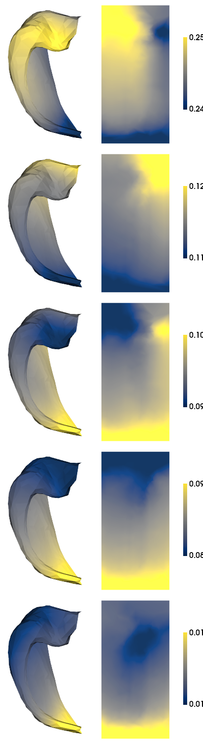
print(f'{np.min(BPhipp_extrapolated, axis=0)} {np.max(BPhipp_extrapolated, axis=0)}')
hm.plotting.surfplot_canonical_foldunfold(BPhipp_extrapolated, den=den, hemis=['L'], labels=labels, unfoldAPrescale=True, tighten_cwindow=True, cmap='cividis', share='row', color_bar='right', embed_nb=True)
[0.23501497 0.10851331 0.096561 0.0804276 0.01657801] [0.25815761 0.12126428 0.11382142 0.10067539 0.02143464]
[17]:
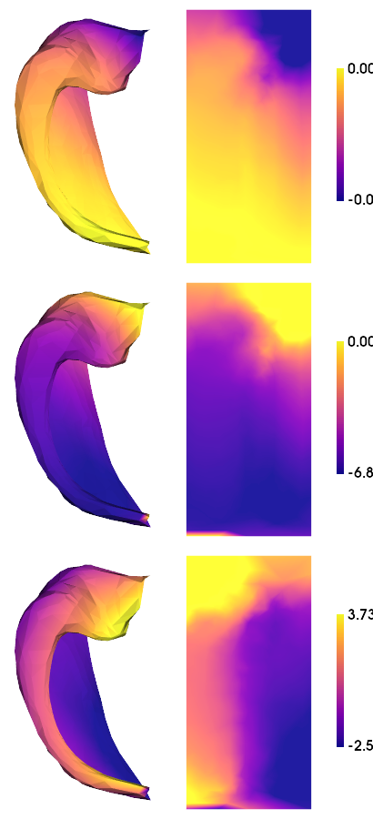
2) Summarize data according to primary gradients
Dimensionality reduction allows us to summarize many maps as primary components, or Gradients. Here we will use BrainSpace to compute nonlinear Gradients using diffusion map embedding. Briefly, this typically consists of computing an affinity matrix (e.g. a correlation between all maps) and then grouping them into a few consistent patterns (Gradients). This allows us to use all aspects of the PSD rather than simplifying it into band powers.
[18]:
# gradient decomposition of power spectrum densities across hippocampal vertices
nGrads = 3
GMpsd = GradientMaps(kernel='pearson') # Here we apply Pearson's R to compute affinity matrices to match the examples of structural MPC gradients
GMpsd.fit(PSDhipp_extrapolated)
[18]:
GradientMaps(kernel='pearson')In a Jupyter environment, please rerun this cell to show the HTML representation or trust the notebook.
On GitHub, the HTML representation is unable to render, please try loading this page with nbviewer.org.
GradientMaps(kernel='pearson')
[19]:
# As above, we can make a nice plot for each of the resulting gradients
hm.plotting.surfplot_canonical_foldunfold(GMpsd.gradients_[:,:nGrads], den=den, hemis=['L'], labels=labels, unfoldAPrescale=True, tighten_cwindow=True, cmap='plasma', share='row', color_bar='right', embed_nb=True)
[19]:
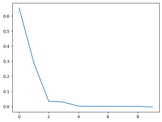
[20]:
# we can also see the lambda value (or eigenvalue) for each gradient
plt.plot(GMpsd.lambdas_/np.sum(GMpsd.lambdas_))
print(GMpsd.lambdas_/np.sum(GMpsd.lambdas_))
[ 6.54620851e-01  2.88111499e-01  3.35005507e-02  2.78776268e-02
  7.51504310e-04  2.18989036e-04  1.10026738e-04  1.74326667e-05
  3.74581429e-06 -5.21222636e-03]
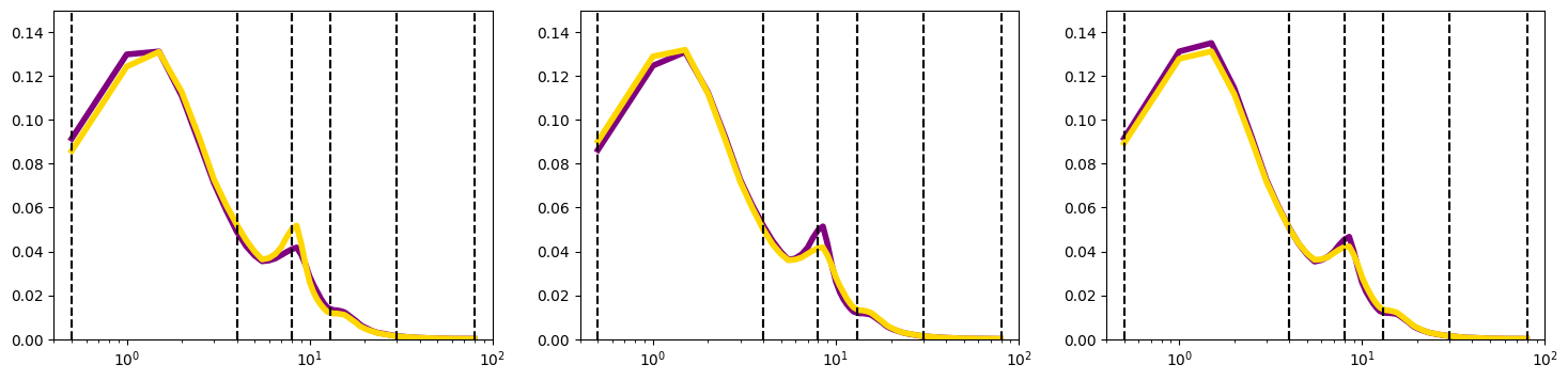
To help contextualize how these gradients relate to PSDs, we can plot the PSDs from only to top and the bottom 10% vertices for each gradient.
[21]:
# compare top to bottom
fig, ax = plt.subplots(nrows=1, ncols=nGrads, figsize=(6*nGrads,4))

for c in range(nGrads):

    nvertsplit = int(nV*.1)

    bot = np.argpartition(GMpsd.gradients_[:,c],nvertsplit)[:nvertsplit]
    top = np.argpartition(GMpsd.gradients_[:,c],-nvertsplit)[-nvertsplit:]

    ax[c].plot(sampspace,np.mean(PSDhipp_extrapolated[top,:],axis=0),color='purple', linewidth=4)
    ax[c].plot(sampspace,np.mean(PSDhipp_extrapolated[bot,:],axis=0),color='gold', linewidth=4)
    #ax[c].set_yscale('log')
    ax[c].set_xscale('log')
    ax[c].set_xlim(0.4,100)
    ax[c].set_ylim(0,.15)
    ax[c].vlines(band_lims.flatten(),ax[c].get_ylim()[0],ax[c].get_ylim()[1],colors='k',linestyles='--')
save
[22]:
# save a copy of the 2D map
!mkdir -p ../maps/HippoMaps-initializationMaps/Dataset-MICs+Frauscher/
for b,band in enumerate(bands):
    cdat = BPhipp_extrapolated[:,b]
    data_array = nib.gifti.GiftiDataArray(data=cdat.astype(np.float32))
    image = nib.gifti.GiftiImage()
    image.add_gifti_data_array(data_array)
    nib.save(image, f'../maps/HippoMaps-initializationMaps/Dataset-MICs+Frauscher/iEEG-BandPower-{band}_average-{nL+nR}_hemi-mix_den-{den}_label-{label}.shape.gii')
[23]:
# save a copy of the 2D map
!mkdir -p ../maps/HippoMaps-initializationMaps/Dataset-MICs+Frauscher/
for l,label in enumerate(labels):
    cdat = GMpsd.gradients_
    data_array = nib.gifti.GiftiDataArray(data=cdat.astype(np.float32))
    image = nib.gifti.GiftiImage()
    image.add_gifti_data_array(data_array)
    nib.save(image, f'../maps/HippoMaps-initializationMaps/Dataset-MICs+Frauscher/iEEG-BandPower-G1to5_average-{nL+nR}_hemi-mix_den-{den}_label-{label}.shape.gii')
[24]:
end_time = time.time()
duration = end_time - start_time
print(f"Total duration: {duration:.2f} seconds")
Total duration: 71.26 seconds